Approximating the shear zone in split bottom granular material simulations using accurate function fitting ↩

aliases: []
shorthands: {}
created: 2022-07-11 10:15:15
modified: 2022-07-11 10:54:07

The assumptions are the same, the shear zone is perpendicular to the axis and the shearing happens in the direction, just like in the simulations of January 2022.

Here, the Python function for approximating the component of the velocity changes to the following:

def vel_accurate_estimator_func(coord, transition_rate, t_rate_lin_x, t_rate_quad_x, t_rate_lin_z, t_rate_quad_z, y_displacement, x_lin, x_quad, z_lin, z_quad):
    x = coord[0]
    y = coord[1]
    z = coord[2]
    t_rate = transition_rate + t_rate_lin_x * x + t_rate_quad_x * x*x + t_rate_lin_z * z + t_rate_quad_z * z*z
    return np.tanh(y_displacement + (y + x*x_lin + x*x*x_quad + z*z_lin + z*z*z_quad)*t_rate)

As we can see, the transition_rate parameter is just a baseline for the t_rate variable, which changes in space as a function of x and z, a second order polynomial.

Corresponding to this, we also have to change the derivative approximator function to get the gradient:

def vel_accurate_estimator_func_derivative_y(coord, transition_rate, t_rate_lin_x, t_rate_quad_x, t_rate_lin_z, t_rate_quad_z, y_displacement, x_lin, x_quad, z_lin, z_quad):
    x = coord[0]
    y = coord[1]
    z = coord[2]
    t_rate = transition_rate + t_rate_lin_x * x + t_rate_quad_x * x*x + t_rate_lin_z * z + t_rate_quad_z * z*z
    return t_rate * (1 - vel_accurate_estimator_func(coord, transition_rate, t_rate_lin_x, t_rate_quad_x, t_rate_lin_z, t_rate_quad_z, y_displacement, x_lin, x_quad, z_lin, z_quad)**2)

From this, we can easily get the fitting parameters using scipy's curve_fit function:

import scipy
from scipy import optimize

fitParams, fitCovariances = optimize.curve_fit(
    vel_accurate_estimator_func, [coords[:, 0], coords[:, 1], coords[:, 2]], vs[:, 0])

And can get the gradients in each particle positions as well:

gradient_from_fit = -vel_accurate_estimator_func_derivative_y(
        [coords[:, 0], coords[:, 1], coords[:, 2]], *fitParams)

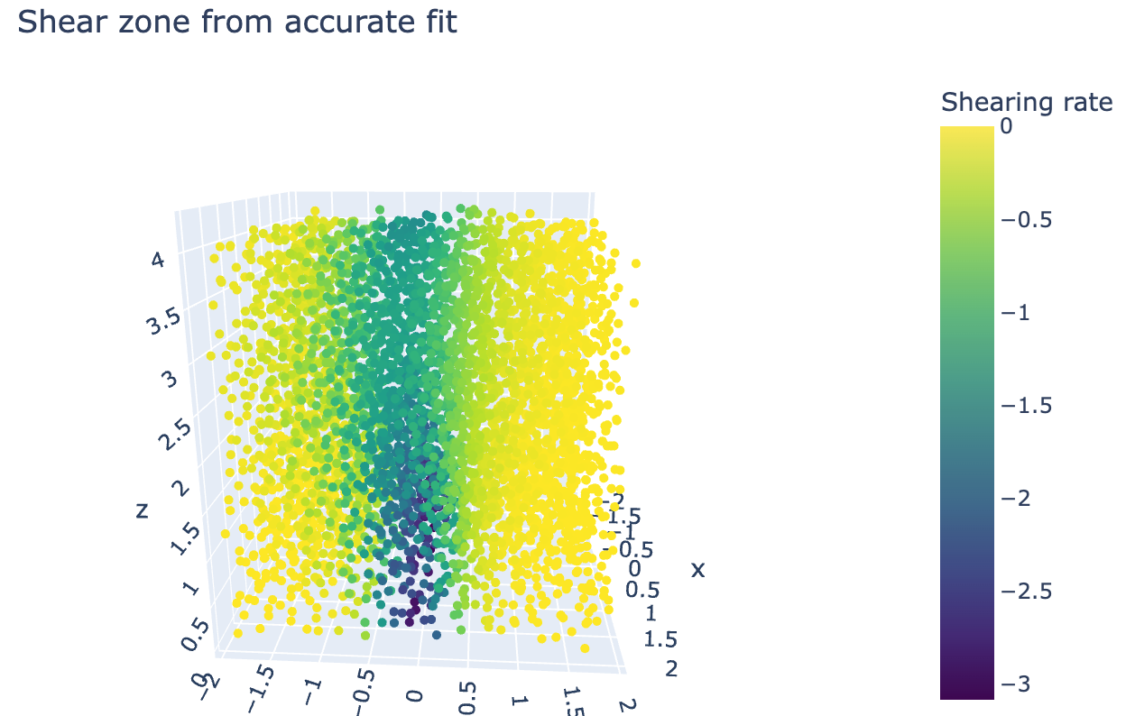
Plotting this, we get:

fig = go.Figure(data=[go.Scatter3d(x=coords[:, 0], y=coords[:, 1], z=coords[:, 2],
                                   mode='markers',
                                   marker=dict(
    size=3, color=(gradient_from_fit),
    colorbar=dict(title="Shearing rate"),
    colorscale='Viridis',
    showscale=True))])
fig.update_layout(width=650, height=400, margin=dict(
    l=0, r=0, b=0, t=40), title="Shear zone from accurate fit")
fig.show()

As we can see, the approximation not only follows the shape of the shear zone, but the width is estimated as well!

Now if we again exclude everything except the shear zone, we get the following:

zone_filter = gradient_from_fit < -1.3

fig = go.Figure(data=[go.Scatter3d(x=coords[:, 0][zone_filter], y=coords[:, 1][zone_filter], z=coords[:, 2][zone_filter],
                                   mode='markers',
                                   marker=dict(
    size=3, color=(gradient_from_fit[zone_filter]),
    colorscale='Viridis',
    colorbar=dict(title="Shearing rate"),
    showscale=True))])
fig.update_layout(width=650, height=400, margin=dict(
    l=0, r=0, b=0, t=40), title="Shear zone from accurate fit, everything else excluded", scene_aspectmode='cube')
fig.update_layout(
    scene=dict(
        xaxis=dict(range=[-2, 2],),
        yaxis=dict(range=[-2, 2],),
        zaxis=dict(range=[-0, 4],))
)
fig.show()

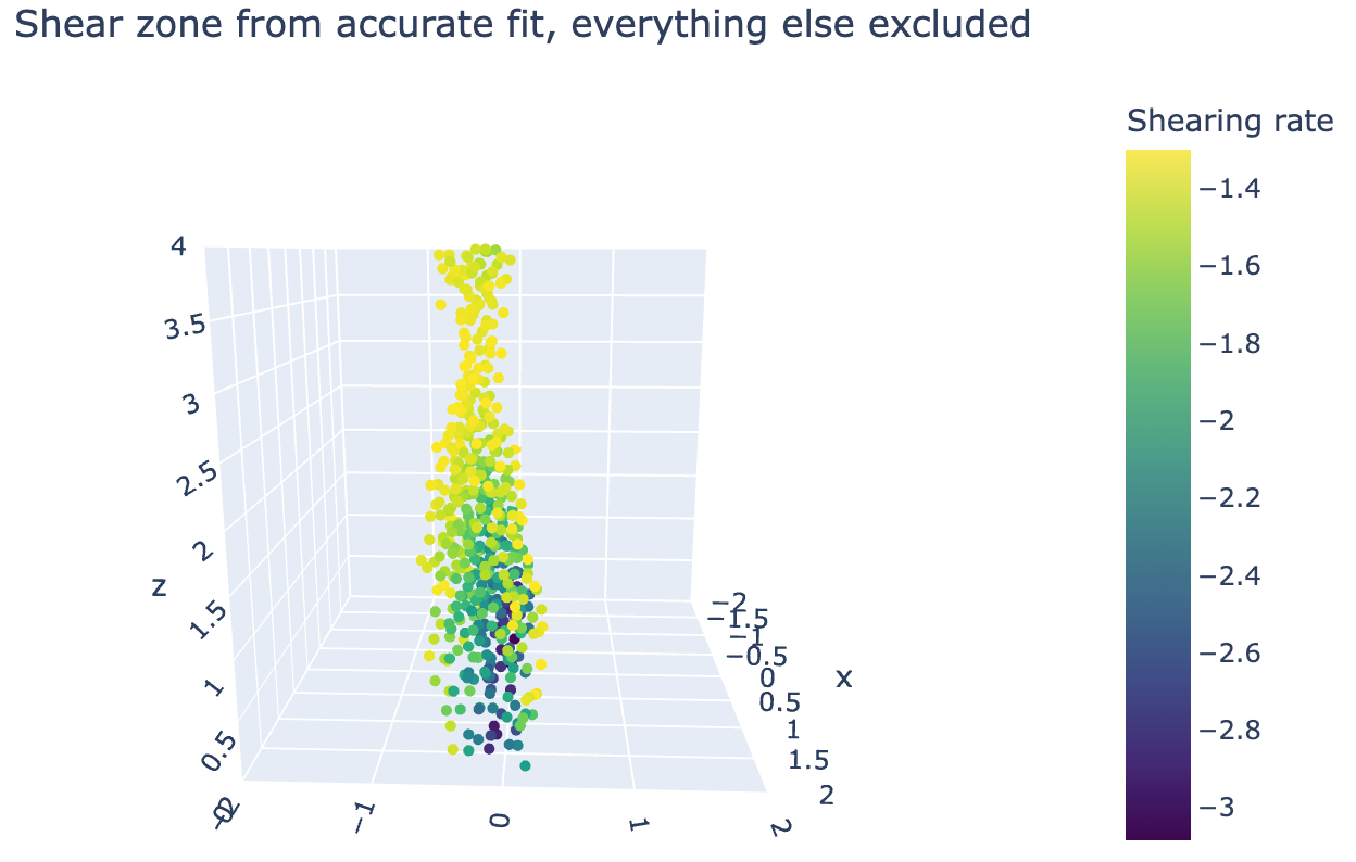
It's easy to see that this really accommodates for the rate at which the two sides of the material transition, which makes filtering the shear zone harder, causing inconsistencies.

Pros and cons

Pros

• Accommodates for the spatial changes in the width of the shear zone

Cons

• Makes the filtering of the shear zone harder than in the simpler method